So I took CS5330 a randomized algorithms course this semester in NUS taught by Prof. Seth Gilbert. The course content in itself is nothing short of beautiful.

I will be describing the broad things I could take away from the course. All the material + my notes for the course can be found here
Note - I was one of the average students in the course, so don’t consider these as the only possible learnings from this course. In case you are already acquainted with this stuff just read up this blog post recommended by our prof. It is the tl;dr version.
- Inequalities:
- We are taught a LOT of inequalities, this image consists of all those that were taught and useful.
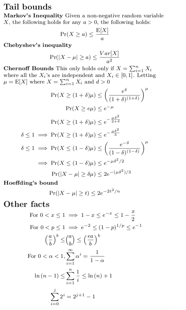
- We have probabilities inequalities in this course like Union Bound, Markov, Chebyshev and Chernoff. These are taught and applied aggressively throughout the course. One imp. thing to note is that if you are bad at a Probability course like MA2216 because you aren’t good with pdf/join distributions/proofs for continuous distributions like Gaussian, Poisson, etc. then it shouldn’t affect your performance in this course, since here the R.Vs are generally Bernoulli or binomial in most cases AND often we are not trying to get a precise answer for a probabilistic event, instead we are always trying to bound it. Getting a hang of where to add/drop stuff when trying to bound things algebraically is a skill that one picks up during this course and which is quite hard to become good at.
- We also exploit this kind of algebraic structure a lot in the course: \((1 - \frac{1}{n})^{n * c \log{n}} \leq e^{c * \log{n}} \leq \frac{1}{n^c}\), where c is a small positive integer.
- We are taught a LOT of inequalities, this image consists of all those that were taught and useful.
- Min-Cut Kargers: An elegant algorithm to do min-cut. Key Insights were \(\rightarrow\)
- If a problem of size \(N\) (in this case finding min-cut of a graph of size \(N\)) can be shrunk to a problem smaller in size (in this case to the size of \(\frac{N}{\sqrt{2}}\) with a decent success probability (here it is \(0.5\)), then instead of decomposing the problem like a straight chain, i.e to go from \(N \rightarrow \frac{N}{\sqrt{2}} \rightarrow \frac{N}{2} \rightarrow \ldots\), and keep on reducing the success probability from \(\frac{1}{2} \rightarrow \frac{1}{4} \rightarrow \frac{1}{8} \rightarrow \ldots\) (almost 0). We can instead do branching :)
- Branching here refers to this: Let us define \(f(N)\) to be the solve function for the problem of size \(N\) which returns the min-cut. Then instead of the chain method where we go from \(f(N) \rightarrow f(\frac{N}{\sqrt{2}})\), now we will do something like this \(\rightarrow\)
- \(f(N) = \min(f(\frac{N}{\sqrt{2}}), f(\frac{N}{\sqrt{2}}))\), i.e call two instances of smaller size and take the better answer. (Note - both of them initially work on the same graph of size \(N\), but because of randomness they will be contracting edges randomly, i.e the two instances of size \(\frac{N}{\sqrt{2}}\) being called, won’t be clones of one another)
- Now analyzing this branching process you can realize that it has \(2*\log{N}\) layers in the recursion tree and each layer has doubled the nodes of the previous layer. The analysis is similar to a merge-sort algo and slightly slower than the chaining method. BUT the benefit in this approach comes from the fact that the probability of correctness is amplified hugely. Effectively now the success probability of the algorithm = probability that there is at least one path from the root to leaf in the recursion tree that has all success edges, where you can traverse an edge downwards successfully with a probability of \(\frac{1}{2}\). This gets lower bounded by \(\geq \frac{1}{depth} \geq \frac{1}{\log{N}}\) (using a non-trivial tree analysis argument), which is MUCH better than earlier success odds of \(\frac{1}{2^{2\log{N}}} = \frac{1}{N^2}\).
- A nice argument is also shown that there can at most be \(N^2\) distinct min-cuts because success probability of Karger’s algo for a specific min-cut is at least \(\frac{1}{N^2}\), so if you add it up for all distinct min-cuts it shouldn’t exceed \(1\), therefore #distinct min-cuts \(\leq N^2\).
- QuickSort Analysis:
- Two ways to analyze the expected complexity. An interesting thing to learn was that JUST commenting on Expected Time Complexity of an algorithm is NOT enough to say it is a good/fast algorithm. Think about plotting Time taken (y-axis) vs Probability (x-axis) graph, it can happen that the tail doesn’t fall rapidly in this graph, so although mean is low, but there is enough variance that often your algo runs super slowly.
- I tried to think of an algorithm with this kind of slowness, but I think it is hard to formalize such a case.
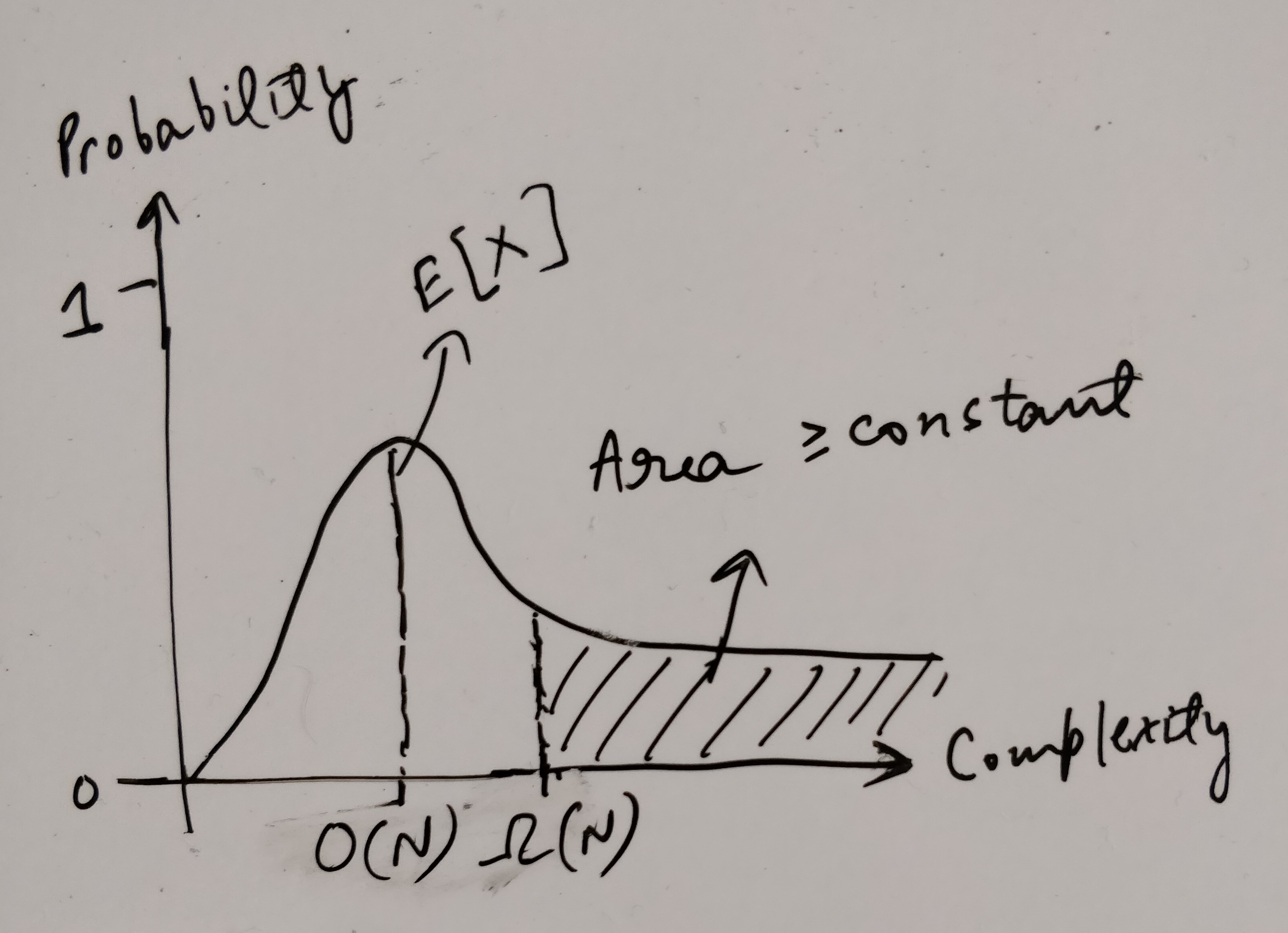
- Because if this happens then \(E[X]\), no longer remains in \(O(N)\) and instead goes up, since \(constant * \Omega{(N)}\) also contributes to \(E[X]\)
- Therefore we also analyze with what probability is the time complexity far away from the mean and try to show that this is very low. Aka \(\Pr(X \geq c*N\log{N}) \leq \frac{1}{N^c}\).
- The insight was, that just like in statistics, the mean of a distribution is NOT an idle way to boil down all the information about the distribution, similarly here just boiling down all the information to \(E[X]\) and commenting about it is NOT enough to be confident about the algorithm.
- Additional References: Must read, about a unifying way to view mean, median, mode of a given statistic
- Stable Matching:
- Not a big topic. We were primarily introduced to deferred decision making and stochastic domination. The problem in itself was put forward as a Balls and Bins problem.
- Stochastic Domination although a simple concept, turns out to be very powerful when analyzing something. It basically comments that instead of analyzing a complicated probabilistic event we upper bound that event by a simpler one and analyze the simpler one.
- Example: Algorithm \(A\) is successful with probability \(\frac{x}{N}\), where \(x\) is some complicated function of \(N\). But you know \(x \geq \frac{N}{2}\). Then just say let us be pessimistic and say that it is successful with probability \(\frac{1}{2}\) exactly. Then if for this simpler algorithm we realize that it runs in \(N\log{N}\) with high probability, then we CAN SAY that Algorithm \(A\) definitely runs in at most \(N\log{N}\) with same high probability.
- Additional References: Wiki link for stochastic domination
- Hashing:
- Open chaining is reduced to a balls and bins problem and analyzed using that.
- Linear Probing has a somewhat hard analysis to grasp. The intuition of making a binary tree to define clusters is still not super clear to me.
- I guess one of the key points is \(E[COST] \leq \sum_{k = 1}^{N}k * \Pr(\text{an elt. is in a cluster of size }K)\\ \leq \sum_{l = 0}^{\log{N}}2^{l + 1} * \Pr(\text{an elt. is in a cluster of size }[2^l, 2^{l + 1}])\)
- Now we show \(\Pr(\text{an elt. is in a cluster of size }[2^l, 2^{l + 1}])\) is small, that is exponentially decreasing with \(l\). To show this we need 4th-moment inequalities and a non-trivial/magical idea involving a “binary tree” and “crowded contiguous segment definition”. I am still unclear as to why we need all these components for the proof to go through and still in the process of trying to understand this portion.
- Flajolet Martin:
- Perhaps the MOST insane algorithm I have ever seen. The algorithm is like super short and has just 3 - 4 steps mainly. But as a competitive programmer, the magical thing is it enables you to “COUNT NUMBER OF DISTINCT ELEMENTS IN A STREAM/ARRAY USING A MIN FUNCTION AGGREGATION”. Obviously, it has two parameters for controlling the algorithm. Firstly, to improves its closeness to optimal answer in terms of delta and secondly the error probability with which it does not fall into the delta range. From a practical competitive programming standpoint, the algorithm is slightly redundant since it requires a lot of runs to reduces both these errors to enable it to pass on online judges. But still, its idea is super fascinating.
- We discuss the FM algorithm, then FM+ which takes the average of a lot of instances of the FM algorithm.
- This averaging of a lot of results is USEFUL in reducing the variance of the algorthm and thus making delta smaller. (This concept is somewhat more general in CS and equivalent to why people use random forests over decision trees in ML-algorithms to reduce variance in their results)
- Then we make FM++ algorithm, which runs a lot of instances of FM+ and sort all the answers and returns the median. This is done because for the median to go bad (i.e lie in error region), at least more than HALF of the FM+ runs need to go bad. Since in FM+ we control the bad probability by some constant (ex. in lecture we used \(\frac{1}{4}\)). Now effectively the FM++ will fail only if more than half of the runs give a bad result. This we can see intuitively, decreases exponentially with the number of runs of FM+ we do. It is kind of like saying you have a coin which with probability $\frac{1}{4}$ gives HEAD and with remaining gives TAILS. Then what is the probability that more than 50% of the times in a run of \(K\) tosses it gives HEADS. This can be seen to decrease exponentially with \(K\) using Chernoff Bound.
- The prof also told us that this “FIRST MEAN, THEN MEDIAN” technique is more of a general technique in randomized algos and also tested this in the midterm examination.
- Additional References: Increment counter algorithm, with a similar idea, tested for midterm
- Min Set Cover:
- Model the problem as ILP (Integer Linear Programming) Problem. Then hand wave and say ILP is ALMOST Like LP. Use LP solver as a black-box. But wait…now the solutions are real numbers and not integers, so you use ROUNDING to get the results. Here rounding the number naively might not be good and the way you round your results is problem specific. In the case of Set Cover the prof showed us a specific rounding method which worked. Using that rounding method he showed that the algorithm gives a valid answer with probability \(1-\frac{1}{e}\), which is although reasonably high, but constant. NOTE - This is NOT the probability of being OPTIMAL, but instead of just giving a VALID SET COVER.
- Now the interesting issue is that if you think we might be able to do something like Karger branching / FM++ and combine multiple runs of this algo to increase this probability then you are correct, HOWEVER, there is no method to merge the answers which keep the answer small. So what you do is RUN this instance \(\log{N}\) times and take the union of all the sets found, which increases the VALID SET COVER probability exponentially, thus making the algorithm work w.h.p (with high probability), however, the answer NO LONGER REMAINS CLOSE TO OPTIMAL. Instead, the union of \(\log{N}\) instances effectively makes the size of the set cover = \(\log{N}\) * (size of the optimal set cover).
- An interesting thing to note here is that this shows you don’t get a linear approximation of min set cover (optimization version is in NP-Hard) by using Randomized Algorithms. You can get a logarithmic factor approximation of this problem with very high probability.
- Random Walks and Expert Learning:
- All these techniques are fairly advanced as compared to the topics discussed above and the fact that we did not have problem sets on these (all these topics are post week7-week8) highlight the fact that some technicalities in these lectures were hand-waved OR not meant to be understood completely by an average Joe like me. So I don’t think I am in a spot to give any insights on these topics.
- Probabilistic Methods:
- This semester the prof did not go through this topic, however, if you search on the internet it is a somewhat standard topic in many randomized algorithm courses. The problem that the probabilistic method tries to tackle is to comment on the existence / bound of a certain deterministic thingy using probability argument.
- Example: Just above at point 1. We see that Karger’s algorithm shows us a side-result that the number of distinct min-cuts is bounded by \(N^{2}\), this is an example of a probabilistic method use case.
- Another example that one can try out is to show that a 3-SAT problem with \(k\) clauses will have at least one solution instance which satisfies \(\geq \frac{7}{8}k\) clauses.
- Additional References: MAX-3SAT Notes from another uni
Conclusion: The course structure is amazing and they teach a lot of good stuff. Prof. Seth Gilbert explains these algorithms very intuitively and you understand the feel of how the inequalities and math should work out after a few of his lectures. As for the grading component this semester, the module primarily consisted of Problem Sets, Midterm, Experimental Project and an Explanatory Paper on a randomized algorithm related research topic. The module does not have a final exam, so…the Random Walks and Expert Learning portion is NOT really graded anywhere.