Information Cascading

Herd mentality meets game theory

In my class on “Incentives in CS”, one of the most interesting concepts I came across was on information cascading. This post attempts to describe the concept by discussing improving iterations over a toy-example.

We encounter many settings where individuals rely not just on their own observations but also on others’ decisions to make assessments. For instance, in the stock market, investors use public signals (e.g., others’ buying/selling behavior) to make decisions. While this “collective intelligence” often works, it can fail when reliance on others creates a bad feedback loop, known as an information cascade

This can be observed especially in social settings where the reward of a decision is delayed substantially but the decision a person took is known immediately to everyone.

Take this example: A group of your friends is planning to RSVP for a party. Knowing your friends likely researched on the worthiness of the experience, you might think, “Well, I don’t think paying X$ and spending Y hours on Friday night is worth-it, but Alice and Bob must have looked into it too and still decided to go, so I’ll trust the majority and RSVP too”. Now, seeing your RSVP, another friend might think, “Hey, let me RSVP as well since Alice, Bob and Claire are all going, and they probably put as much thought into this as I would.” And so, the cascade continues. How many times have your RSVP’d to a party in FOMO trusting the majority?

Let’s analyze a simpler yet concrete example

Setup

Imagine a game¹ where there is single box that either contains:

• 2 blue and 1 red ball (Type B), or

• 1 blue and 2 red balls (Type R).

The box being of either type has an equal probability (50%).

Now there are \(N\) players (take \(N\) ~ 1 million) in a queue, where each of them turn-by-turn:

• Privately draw a ball from the box at random, note its color, and put it back in.

• Report publicly whether they believe the box is Type B or Type R.

• Future players hear all previous guesses.

Version 1

Say each player at the end of the game, gets 1\$ if they had reported correctly and 0\$ if they had not. What would be the optimal play for each player individually? Also if everyone plays optimally, what would be the expected total payout received by the N players?

Also as a side-quest, if you were one of the players, would you stand near the front or towards the back of this queue. A low stakes squid game edition it is!

… [I would suggest thinking for ~5-10 mins]

Starting from Player 1 all the way to Player N, you can think about the decisions as a decision tree with the information shown (Figure 1).

Notation: P1 refers to Player 1, P2 refers to Player 2 and so on

We observe P1 uses the information that they sampled and P2 uses combined information of P1 + P2, thus making sensible decisions.

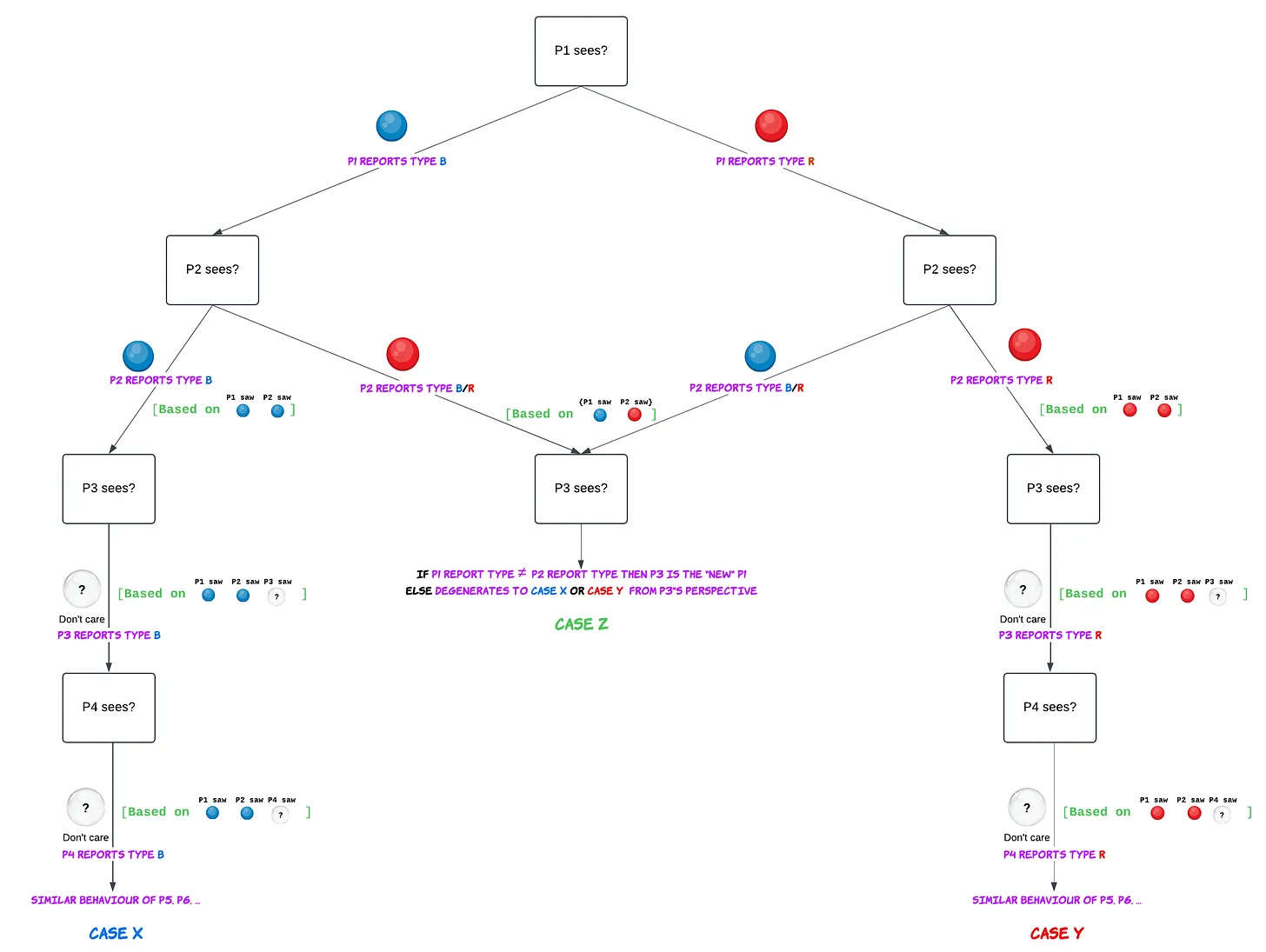
From P3 onwards we see Case X where P1 and P2 saw same color (say Blue) however P3 saw opposite color (fill in ? = Red in your mind), even then P3 would think its more likely to be type B². The *issue* with this is, P4 can no longer know if P3 saw a Blue or a Red ball, because they know P3’s optimal play in either case was to guess type B, so the actual information P4 has is only of the balls sampled by P1 + P2 + their own. Similarly for all the subsequent players they would only look at the actual information provided by P1 + P2 + their own and irrespective of what they see themselves, they would stick with what P1 + P2 saw. This is the cascade we are talking about.

So in Case X and Case Y we observe that everyone guesses correctly if P1 and P2 saw the dominant color (has 4/9 chance) but everyone guesses wrongly if on the off-chance they both saw the minority color (has 1/9 chance). In the remaining cases (denoted by Case Z) P1 and P2 report different types³ and so for P3 the information collected by P1 and P2 effectively “cancels out” and we can induct on a game of $N - 2$ players.

Let f(n) denote the expected payout of n players combined, then

\[f(n) = \frac{4}{9}n + \frac{1}{9}0 + \frac{4}{9}(1 - f(n - 2)), f(0) = 0 \Rightarrow f(n) \approx 0.8n\]

So the expected payout is 0.8n⁴.

How about calculating the probability of being correct for each player? We can approximate the case where we keep seeing (Blue, Red) pair (unordered) consecutively for every two players is highly unlikely (exponentially decreasing probability), therefore with high probability after the first couple of even number of rounds, there will be a strict majority of red samples or blue samples following which the crowd will stick with that majority, i.e. let Pr(Success) denote the probability that the players converge to the correct type, then:

\[Pr(Success) = \frac{4}{9} + \frac{4}{9}Pr(Success) + \frac{1}{9}0 \Rightarrow Pr(Success) = 0.8\]

Notice how the number of players being too many or too few in the game is not playing any role in Pr(Success).

Also since Pr(Success)⁵ is same across the players at the back, neither are you better off being at the back of the queue (contrary to one’s first instincts).

Version 2

I suggest a change to the current game, to increase sharing of information.

Updated change: Instead of guessing type B or type R, the players will now speak out *loudly* a number $p$ between $[0, 1]$. If the player reports $p$ and the box is of type B, they will get p\$ otherwise they will receive (1 - p)\$ . Our “hope” here is that players are incentivized to report $p$ = the true probability they think the box is of type B.

How will the players play now to maximize their individual “expected” payouts?

… [Thinking time]

Hint: What values of $p$, would maximize the expected payout for P1?

Expand for ugly math proof

$$ {\tiny\begin{align*} E[\text{payout} | \text{sampled B}] &= p Pr(\text{box is of type B} | \text{sampled B}) + (1 - p)Pr(\text{box is of type R} | \text{sampled B})\\ \newline Pr(\text{box is of type B} | \text{sampled B}) &= \frac{Pr(\text{sampled B} | \text{box is of type B)} Pr(\text{box is of type B})}{Pr(\text{sampled B} | \text{box is of type B})Pr(\text{box is of type B}) + Pr(\text{sampled B} | \text{box is of type R})Pr(\text{box is of type R})} \\ &= \frac{2/3 \times 1/2}{2/3 \times 1/2 + 1/3 \times 1/2} = \frac{2}{3}\\ \newline \newline E[\text{payout} | \text{sampled B}] &= \frac{2}{3}p + \left(1 - \frac{2}{3}\right)p\\ &= \frac{1}{3} + \frac{1}{3}p \end{align*}} $$ which is maximized when $p = 1$
Similarly, $$ \tiny{\begin{align*} E[\text{payout} | \text{sampled R}] &= p Pr(\text{box is of type B} | \text{sampled R}) + (1 - p)Pr(\text{box is of type R} | \text{sampled R})\\ \newline Pr(\text{box is of type B} | \text{sampled R}) &= \text{ [Similar Bayes stuff as above]} = \frac{1}{3}\\ E[\text{payout} | \text{sampled R}] &= p\frac{1}{3} + (1 - p)(1 - \frac{1}{3})\\ &= \frac{2}{3} - \frac{1}{3}p \end{align*}} $$ which is maximized when $p = 0$

Gist of the ugly math: Player 1 would always be incentivized to report $p = 0$ or $p = 1$ and no other middle value of $p$.

For the second player, they would have observed the first players’s $p = 0$ or $p = 1$ and know accordingly what they had sampled. So they could update their prior and come up with:

\[Pr(\text{box is of type B} | \text{P1 sampled color A and P2 sampled color B}) = c\]

where c is some constant that would be > 1/2 if {A, B} both are Blue, < 1/2 if {A, B} both are Red and = 1/2 if one is Blue, one is Red.

We need not worry about the exact constant, eventually it will lead to:

\[\begin{align*} E[\text{payout} | \text{P1 sampled color A and P2 sampled color B}] &= pc + (1 - p)(1 - c)\\ &= p(2c - 1) - c + 1 \end{align*}\]

since this is linear in $p$, with slope $2c - 1$. So it ends up being a straight line graph (See sketch below) which would maximize at either $p = 0$ or $p = 1$ for the range $[0, 1]$, depending on the sign of the slope (i.e. $2c - 1 > 0$ or not? == $c > 1/2$ or not?)⁶

The first two players reporting only values $p = 0$ or $p = 1$ devolved the information for the subsequent players to the same information as they received in Version 1.

So in case of seeing $p = 1$ twice, P3 knows that P1 and P2 both saw Blue, so irrespective of what they sample, be it Red or Blue, for them Pr(box is of type B | what P3 knows) > 1/2

This makes their payout look like:

\[E[\text{payout} | \text{what P3 knows}] = pc + (1 - p)(1 - c), c > 1/2\]

Since $c > 1/2$, we know this calculation maximize at $p = 1$. Similarly in the case of seeing $p = 0$ twice, we would get Pr(box is of type B | what P3 knows) < 1/2 which would maximize at $p = 0$.

One can observe that for subsequent players (say $P_x$), they would work out same logic as P3 (and wont be using P3, P4, …, $P_{x-1}$’s decision info) because of the same argument as Version 1.

We introduced Version 2 in the hope that players would be incentivized to report their true beliefs which would further help the system as a whole, however we observed that extreme values of $p = 0$ or $p = 1$ maximize the expected payoff of the linear functions of the form: $pc + (1 - p)(1 - c)$ for an arbitrary constant $c$.

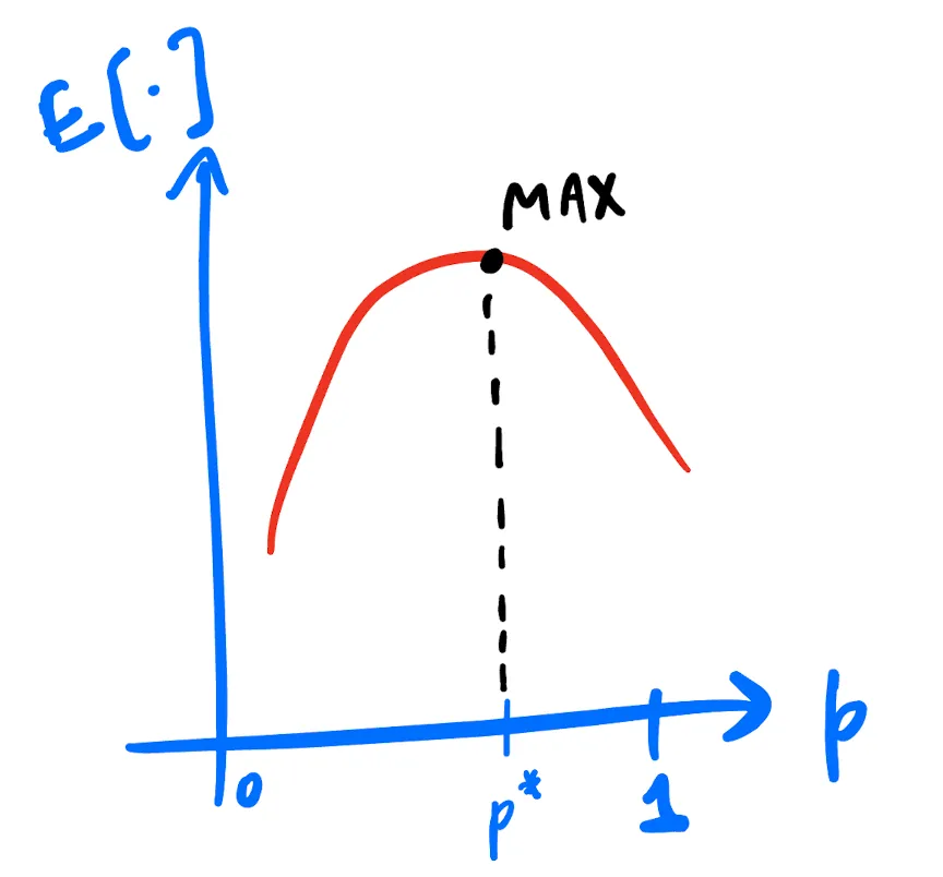
How can we fix our reward function to “actually” incentivize players to report their true probabilities? The instinct should be to make the expected payoff function such that it maximizes at true $p$ value (let this be denoted by $p^{\ast}$). Now such a function would have to maximize at $p^{\ast}$ which is somewhere in the range $[0, 1]$ and be below its maxima for all the other points in $[0, 1]$ (See sketch below). This might incline you to guess some kind of quadratic function or an even higher degree polynomial function.

Version 3

Well the intuition checks out, let us add a regularization term of p(1 - p) to our existing reward function.

So now our reward functions (for type B and type R) are respectively:

\[\begin{align*} u_B(p) &= p + p(1 - p) = 2p - p^2\\ u_R(p) &= (1 - p) + p(1 - p) = 1 - p^2 \end{align*}\]

Assuming $p^{\ast}$ is the true probability that the player believes the box is of type B and the player actually report $p$, we get that it becomes optimal⁷ for the player to report $p = p^{\ast}$ so as to maximize their payout

Expand for math proof

$$ \begin{align*} E[\text{payout}] &= u_B(p)p^{\ast} + u_R(p)(1 - p^{\ast})\\ &= 2pp^{\ast} - p^2p^{\ast} + 1 - p^{\ast} - p^2 + p^2p^{\ast}\\ &= -p^2 + 2pp^{\ast} + 1 - p^{\ast}\\ \Rightarrow \frac{\partial E[\text{payout}]}{\partial p} &= 2p^{\ast} - 2p = 0 \Rightarrow p = p^{\ast}\\ \Rightarrow \frac{\partial^2 E[\text{payout}]}{\partial p^2} &= -2 < 0 \end{align*} $$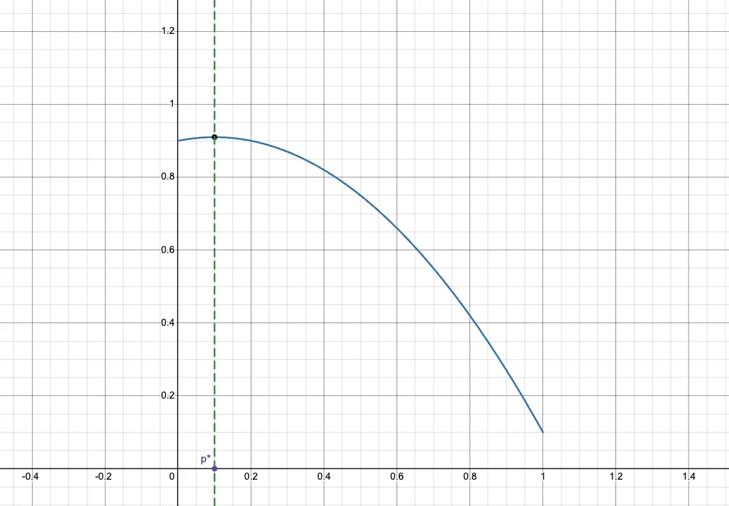

Nice! Our incentives are aligned to make each player report their $p$ honestly which subsequent players can listen to and basically know what each player before them saw.

What would be the expected total payout of this version of the game? It would be ~N. The reasoning is that after the first few samples — say, the first 99 samples, the 100th player would know, based on previous $p$’s what each prior player observed (a red ball or blue ball). By the time around 100 samples have been drawn, the 1/3 and 2/3 split of red and blue balls would become very apparent meaning

Pr(Success for the 100th player) ~ (almost) 1

So standing behind in the queue is better in this version and the payoffs would converge to 1 as well. Notice, however that the regularizer bonus would no longer benefit the latter players and is primarily incentivizing honesty among the first handful⁸ of players.

Conclusion

In essence, we observed how our instincts for the trivial setup of the box problem turned out to be incorrect. We encountered cascade issues, demonstrating that even with a large N, the system as a whole fails to reliably discover the type of the box. By making the reward function more “complex,” we incentivized players to share their true p*, thereby getting a quick convergence on the correct answer.

Food for thought #1: Imaging you are the game designer, and the total payout for this game comes from your pocket. With a budget of N\$, how do you run the Version 3 game within this limited budget? Note that the regularizer bonus also comes out of your pocket, potentially leading to an expected cost of N + O(logN)\$ which you don’t have. Think of some ways (even trivial ones), on how you would change the reward functions to stay within budget?

Food for thought #2: When a couple of influencers tweet about a meme coin, can these influencers—aka early adopters—trigger a cascade, where the general public perceives it is a good investment (even though, in a vacuum, their assessment might suggest otherwise) merely because the early adopters broadcasted it as such? In such a scenario, is it off-chance that the early adopters mis-assessed the opportunity, or is their reward function fundamentally different from that of the general public?

Incentives shape behavior, as we’ve seen throughout this post. Understanding them is essential to designing systems that align individual actions with collective goals.

“Show me the incentive and I’ll show you the outcome” - Charlie Munger